Issues in Earth Science
“Eww, There’s Some
Geology in my Fiction!”
Issue 2, Nov 2014
Teacher Resources
Suggestions for Activities and Discussions to accompany a Reading of
Plate Tectonics and Non-Platonic
Relationships by Alicia Cole
Curriculum for the
Earth Sciences often includes the Theory of Plate Tectonics as a key element,
and often presents Plate Tectonics as the conceptual model for students to hang
their new ideas on. However, learning
facts and theories in and of itself is not the goal of the Next Generation
Science Standards (NGSS). The practices
of science, one of three components of learning called 'dimensions of learning'
in the NGSS, involve learning how to figure things out—doing science--not
merely accepting the facts and theories that someone else has figured out for
you. The theory of plate tectonics is a great place
for students to consider the various lines of evidence that support this
particular scientific theory.
A good starting place
for examining evidence with your students is to plot the locations of
earthquakes. The epicenters aren’t
distributed randomly but predominantly occur in narrow bands, marking the locations
where plates meet. Maps showing an
earthquake plotting activity to find plate boundaries are found at http://web.mnstate.edu/colson/est/est2b6.html.
You can also examine other
lines of evidence such as locations of volcanic activity, the age of the ocean
floor, and seafloor topography. Below
are some suggested data-driven activities that you can do with your student to
engage them in the practices of science as they relate to the different types
of plate boundaries mentioned in Plate
Tectonics and Non-Platonic Relationships.
Many of these suggested
activities, along with comprehensive teacher and student resources, may be
found at Tectonics, which is part of the Environmental
Literacy and Inquiry (ELI) site at
Lehigh University. The six
investigations at this site form a coherent instructional sequence in which students consider the data and evidence for
the different kinds of boundaries and the multiple lines of evidence that
support the theory of plate tectonics. This
online resource
provides teacher guides, classroom-ready investigations for students and detailed
‘how-to’ supports for using the different map layers included in each of the
investigations.

Convergence with Subduction
No one has ever seen a subducting plate deep under a mountain range. Sadly, there are no Mole Machines that allow us to go there in real life. So how do we know that subduction zones even exist? One line of evidence that you can examine and consider with your students is the increasing depth of earthquakes as one goes farther inland from a deep ocean trench.
Investigation 6 at ELI guides
students in exploring earthquake depth and viewing slab profiles across the
Aleutian Islands. Below are two sample maps (from the Investigation 6 online GIS activity), one with earthquake depths along the convergent
boundary and one showing the profile of earthquake depth across the convergent
boundary.

Depth of earthquakes
are color coded in this map image.
Notice how the earthquakes get deeper as you go north away from the
trench where subduction occurs.
Earthquakes occur where blocks of rock are moving relative to each other,
so the location of the quakes mark the course of the descending plate.

The image above shows
the cross-sectional view of Earthquake depth (subduction zone profile), which
can then be used to map the depth of the subducting plate; contour lines are color-coded
on the map with green being shallower depths of the descending plate and red
being deeper depths.
Divergence
Today, we can measure
the relative motion of plates with GPS.
But how did we first discover plate motion before we could make such
measurements, and how do we know that plates have been diverging for millions
of years? Investigation 4
and Investigation 4 maps gives students the GIS map layers and tools to investigate the lines
of evidence for diverging plates. The
measured age of sea floor rock is shown in sample map 1. Sample map 2 includes the topographic profile
of the ocean floor, showing a range of underwater mountains at the divergent
boundary, to compliment the ‘birds-eye’ view of seafloor ages.

The map above shows
the ages of sea floor crust based on values measured at many locations. Notice that the rocks near the divergent
boundary (where new rock would be expected to form if plates truly are
diverging) are younger.

The image above shows
the topographic profile across the divergent boundary at the ridge in the
middle of the Atlantic Ocean along with the map of age of the ocean crust.
Including some simple math, conversions, and testing the theory
In good science,
multiple lines of evidence should support the same ideas and can be used to
check theories and measurements. You
might have your students compare the rate of spreading at the divergent
boundary calculated from the measured age of rocks and width of the Atlantic
Ocean with values derived in modern times by GPS.
Use the measure tool
on the ELI activity (or use an atlas with a scale bar) to measure the distance
across the Atlantic from Africa to the East Coast of North America (for
example, it might come out close to 5500km).
Then consider the age of the rocks on the farthest west and east
portions of the Atlantic (perhaps in the vicinity of 180 million years from the
maps above taken from the ELI activity).
From this, students can calculate a rate of spreading (5500km in 180
million years--which through some unit conversions gives them about 3.1
cm/year, on average).
You can then have students
consider the GPS data below that shows the rate of spreading at the Atlantic
divergent zone where it crosses Iceland.
Points on one side of the divergent zone are moving in one direction
(negative values) and points on the other side are moving in the opposite
direction (positive values). Students
can see that places on one side are moving away at about 1.5cm/year (within a
range of 1-3cm/year) and places on the other side are moving the other
direction at 1.5cm/year (again within a range of 1-3cm/year) for a total
spreading rate of about 3cm/year, providing a reasonably close match to the
rate of spreading averaged over the last 180 million years. This provides an interesting test not only of
the theory of plate tectonics, but at test supporting the accuracy of
measurements of ages of rock in the floor of the Atlantic Ocean.
Some students might
be ready to think about uncertainty. Uncertainty
in the measurements are indicated by error bars. Notice that the variation in measurements for
any one data collection period stays within the uncertainty bars and that the
data with larger uncertainty bars also has greater variation from one
measurement to another. However,
different collection periods have different average values. Is this due to random chance, or were there
real variations in spreading rate (surges and abatements) during the time
period of GPS measurement? Taking into
account the consistency of the measurements and the error bars, students might
infer that measurements prior to 1993 indicate a faster rate of spreading than
during 1993-2004.
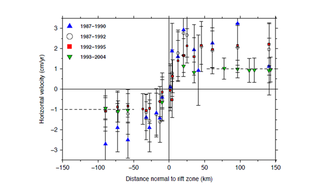
GPS data above are
from "Crustal deformation in Iceland: Plate spreading and earthquake deformation"
by Thóra Árnadóttir, Halldór Geirsson and Weiping Jiang published in JÖKULL No.
58, 2008.
Transform
Investigation 5
and investigation 5 maps allows students to explore the Charlie-Gibbs Fracture Zone and the San
Andreas system. The screen shot below mapping
the age of ocean floor shows the age offset along the transform boundary in the
North Atlantic Ocean. Plate motion
videos, available in one of the data layers, helps students visualize plate
motion and features that result from the motion. You can ask your students "what is the evidence that a transform boundary
exists at this location?"

Continent-Continent Convergence without subduction
Continent-Continent
convergence results in towering mountains like the Himalayas and the Alps, but
since there is no subduction, there are no deep earthquakes. Students can see this by plotting earthquakes
with different depths in the Investigation 6 map activity at ELI (although, there are some complexities around the
edges of the Alps and Himalayas that do result in deeper earthquakes).
Also, with the lack
of subduction comes with a lack of volcanic activity. This is seen if you plot composite volcanoes
on your maps in Investigation 6
map.
Each type of plate
boundary has its own unique set of features.
Shallow earthquakes occur at all of the different kinds of plate
boundaries. Deep earthquakes occur at
convergent boundaries with subduction.
Volcanoes occur at both divergent boundaries and convergent boundaries
with subduction (although the two boundaries are characterized by different
kinds of volcanos). Trenches occur at
convergent boundaries with subduction.
The highest mountains occur at convergent boundaries, either with or
without subduction. PDF maps with the
locations of volcanoes, earthquakes, mountains, trenches and other features can
be found at http://web.mnstate.edu/colson/est/esttectoniclab.html
Connecting to the Next Generation Science Standards
The investigations at the Tectonics site address the science practices of observing patterns, developing and using models, analyzing and interpreting data, and constructing explanations.
These investigations provide a well-integrated instructional sequence that supports learning towards the following performance expectations: MS-ESS2-1, MS-ESS2-2, MS-ESS2-3, MS-ESS3-2, HS-ESS1-5, HS-ESS2-1.

———————————————————————————
The Teacher Resources
for Plate Tectonics and Non-Platonic
Relationships are written by Russ and Mary Colson with thanks to the
excellent NSF-funded Environmental Literacy and Inquiry (ELI) site at Lehigh
University.
Return to
Plate Tectonics
and Non-Platonic Relationships by Alicia Cole
Return to “Eww, There’s Some Geology in My Fiction.”
Find more essays,
games, and stories at
©2014 Issues in Earth
Science